Functional Programming for Deep Learning
Joyce Xu
15 Apr 2019
•
13 min read

Before I started my most recent job at ThinkTopic, the concepts of “functional programming” and “machine learning” belonged to two different worlds entirely. One was a programming paradigm surging in popularity as the world turned towards simplicity, composability, and immutability to maintain complex scaling applications; the other was a tool to teach computers to autocomplete doodles and make music. Where was the overlap?
The more I worked with the two, the more I began realizing that the overlap is both practical and theoretical. Firstly, machine learning is not a stand-alone endeavor; it needs to be rapidly incorporated into complex scaling applications in industry. Secondly, machine learning — and deep learning in particular — is functional by design. Given the right ecosystem, there are several compelling reasons to perform deep learning in an entirely functional manner:
-
Deep learning models are compositional. Functional programming is all about composing chains of higher-order functions to operate over simple data structures. Neural nets are designed the same way, chaining together function transformations from one layer to the next to operate over a simple matrix of input data. In fact, the entire process of deep learning can be viewed as optimizing a set of composed functions, meaning the models themselves are intrinsically functional.
-
Deep learning components are immutable. When functions operate over the input data, the data is not changed, a new set of values are outputted and passed on. Furthermore, when weights are updated, they do not need to be “mutated” — they can just be replaced by a new value. In theory, the updates to the weights can be applied in any order (i.e. they are not dependent on one another), so there is no need to keep track of a sequential, mutable state.
-
Functional programming offers easy parallelism. Most importantly, functions that are pure and composable are easy to parallelize. Parallelism means more speed and more compute power. Functional programming gives us concurrency and parallelism at essentially no cost, making it much easier to work with large, distributed models in deep learning. There are many theories and perspectives regarding the combination of functional programming and deep learning, from mathematical arguments to practical overviews, but sometimes it’s most convincing (and useful) just to see it in practice. Here at ThinkTopic, we’ve been developing an open-source machine learning library called Cortex. For the rest of this post, I will introduce some ideas behind functional programming and put them to use in a Cortex deep learning model for anomaly detection.
There are many theories and perspectives regarding the combination of functional programming and deep learning, from mathematical arguments to practical overviews, but sometimes it’s most convincing (and useful) just to see it in practice. Here at ThinkTopic, we’ve been developing an open-source machine learning library called Cortex. For the rest of this post, I will introduce some ideas behind functional programming and put them to use in a Cortex deep learning model for anomaly detection.
Clojure Basics
Before we continue on our Cortex tutorial, I want to introduce some basics of Clojure. Clojure is a functional programming language that’s really good at two things: concurrency and data processing. Fortunately for us, both of those things are incredibly useful for machine learning. In fact, one of the primary reasons we use Clojure for machine learning is the fact that day-to-day work in preparing datasets for training (data manipulation, processing, etc.) can easily outweigh the work of implementing the algorithms, especially when we have a solid library such as Cortex for learning. Using Clojure and .edn (instead of C++ and protobuf), we can gain leverage and velocity on ML projects.
For a more in-depth introduction to the language, take a look at the community guide here.
On with the basics: Clojure code is made up of a bunch of expressions that are evaluated at run-time. These expressions are wrapped in parentheses, and are typically treated as function calls.
(+ 2 3)          ; => 5
(if false 1 0)   ; => 0
There are 4 basic collection data structures: vectors, lists, hash-maps, and sets. Commas are treated as whitespace, so they are typically omitted.
[1 2 3]            ; vector (ordered)
'(1 2 3)           ; list (ordered)
{:a 1 :b 2 :c 3}   ; hashmap or map (unordered)
#{1 2 3}           ; set (unordered, unique values)
The single quote in front of the list simply prevents it from being evaluated as an expression.
Clojure also comes with many, many, built-in functions to operate over these data structures. Part of the beauty of Clojure is that it was designed to have many functions for very few data types, as opposed to to having a few specialized functions for each of many data types. Being an FP language, Clojure supports higher-order functions, meaning functions can be passed around as arguments to other functions.
(count [a b c])              ; => 3
(range 5)                    ; => (0 1 2 3 4)
(take 2 (drop 5 (range 10))) ; => (5 6)
(:b {:a 1 :b 2 :c 3})        ; use keyword as function => 2
(map inc [1 2 3])            ; map and increment => (2 3 4)
(filter even? (range 5))     ; filter collection based off predicate => (0 2 4)
(reduce + [1 2 3 4])         ; apply + to first two elements, then apply + to that result and the 3rd element, and so forth => 10
Of course, we can also write our own functions in Clojure, using defn. Clojure function definitions follow the form (defn fn-name [params*] expressions), and they always return the value of the last expression in the body.
(defn add2
  [x]
  (+ x 2))
(add2 5)     ; => 7
let expressions create and bind variables within the lexical scope of the “let”. That is, in of the expression (let [a 4] (...)), the variable “a” takes on a value of 4 inside (and only inside) the inner parentheses. These variables are called “locals.”
(defn square-and-add
  [a b]
  (let [a-squared (* a a)
        b-squared (* b b)]
    (+ a-squared b-squared)))
(square-and-add 3 4)       ; => 25
Finally, there are a couple of ways to create anonymous functions, which can either be assigned to a local or passed to a higher-order function.
(fn [x] (* 5 x))          ; anonymous function
#(* 5 %)                  ; equivalent anonymous function, where the % represents the function's argument
(map #(* 5 %) [1 2 3])    ; => (5 10 15)
That’s it for the basics! Now that we’ve learned some Clojure, let’s put the fun in functional programming and get back to some ML.
Cortex
Cortex is written in Clojure, and is currently one of the largest and fastest-growing machine learning libraries that uses a functional programming language. The rest of this post will walk through how to build a state-of-the-art classification model in Cortex, and the functional programming paradigms and data augmentation techniques required to do so.
Data Preprocessing
Our dataset is going to be the credit card fraud detection data provided by Kaggle here. It turns out this dataset is incredibly imbalanced, containing only 492 positive fraud cases out of 284,807. That’s 0.172%. This is going to cause problems for us later, but first let’s just take a look at the data and see how the model does.
In order to ensure anonymity of personal data, all the original features except “time” and “amount” have already been transformed to PCA components (where each entry represents a new variable that contains the most relevant information from the raw data). A little data exploration will show that the first “time” variable is fairly uninformative, so we’ll drop that as we’re reading in the data. Here is what our initial code looks like:
(ns fraud-detection.core
  (:require [clojure.java.io :as io]
           [clojure.string :as string]
           [clojure.data.csv :as csv]
           [clojure.core.matrix :as mat]
           [clojure.core.matrix.stats :as matstats]
           [cortex.nn.layers :as layers]
           [cortex.nn.network :as network]
           [cortex.nn.execute :as execute]
           [cortex.optimize.adadelta :as adadelta]
           [cortex.optimize.adam :as adam]
           [cortex.metrics :as metrics]
           [cortex.util :as util]
           [cortex.experiment.util :as experiment-util]
           [cortex.experiment.train :as experiment-train]))

(def orig-data-file "resources/creditcard.csv")
(def log-file "training.log")
(def network-file "trained-network.nippy")

;; Read input csv and create a vector of maps {:data [...] :label [..]},
;; where each map represents one training instance in the data
(defonce create-dataset
  (memoize
    (fn []
      (let [credit-data (with-open [infile (io/reader orig-data-file)]
                          (rest (doall (csv/read-csv infile))))
            data (mapv #(mapv read-string %) (map #(drop 1 %) (map drop-last credit-data))) ; drop label and time
            labels (mapv #(util/idx->one-hot (read-string %) 2) (map last credit-data))
            dataset (mapv (fn [d l] {:data d :label l}) data labels)]
        dataset))))
Cortex neural nets expect input data in the form of maps, such that each map represents a single labeled data point. For example, a classification dataset could look like [{:data [12 10 38] :label “cat”} {:data [20 39 3] :label “dog“} ... ]. In our create-dataset function, we read in the csv data file, designate all but the last column to be the “data” (or features), and designate the last column to be the labels. In the process, we turn the labels into one-hot vectors (e.g. [0 1 0 0]) based on the classification class, because the last softmax layer of our neural net returns a vector of class probabilities, not the actual label. Finally, we create a map from these two variables and return it as the dataset.
Model Description
Creating a model in Cortex is fairly straightforward. First, we’re going to define a map of hyper-parameters to be used later during training. Then, to define a model, we simply string the layers together:
(def params
  {:test-ds-size      50000 ;; total = 284807, test-ds ~= 17.5%
   :optimizer         (adam/adam)   ;; alternately, (adadelta/adadelta)
   :batch-size        100
   :epoch-count       50
   :epoch-size        200000})

(def network-description
  [(layers/input (count (:data (first (create-dataset)))) 1 1 :id :data) ;width, height, channels, args
  (layers/linear->relu 20) ; num-output & args
  (layers/dropout 0.9)
  (layers/linear->relu 10)
  (layers/linear 2)
  (layers/softmax :id :label)])
network-description is a vector of neural network layers. Our model consists of:
- an input layer
- a fully-connected (linear) layer with the ReLU activation function
- a dropout layer
- another fully-connected ReLU layer
- an output layer of size 2 that is passed through the softmax function.
In both the first and the last layers, we need to specify an :id. This id refers to the key in the data map that our network should look at. (Recall that the data map looks like {:data [...] :label [...]}). For our input layer, we pass in the :data id to tell the model to grab the training data for its forward passes. In our final network layer, we provide :label as the :id, so the model can use the true label to calculate our error with.
Training and Evaluation
Here’s where it gets a little more difficult. The train function itself is actually not so complicated — Cortex provides a nice, high-level call for training, so all we have to do is pass in our parameters (the network, training and testing dataset, etc.). The only caveat is that that the system expects an effectively “infinite” dataset for training, but Cortex provides a function (infinite-class-balanced-dataset) to help us transform it.
(defn train
  "Trains network for :epoch-count number of epochs"
  []
  (let [network (network/linear-network network-description)
        [train-orig test-ds] (get-train-test-dataset)
        train-ds (experiment-util/infinite-class-balanced-dataset train-orig
                                            :class-key :label
                                            :epoch-size (:epoch-size params))]
    (experiment-train/train-n network train-ds test-ds
                                      :batch-size (:batch-size params)
                                      :epoch-count (:epoch-count params)
                                      :optimizer (:optimizer params)
                                      :test-fn f1-test-fn)))
The complicated part is the f1-test-fn. Here’s the thing: during training, the train-n function expects to be provided with a :test-fn that evaluates how well the model is performing and determines whether or not it should be saved as the “best network.” There is a default test function that evaluates cross-entropy loss, but this loss value is not so easy to interpret, and it doesn’t suit our imbalanced dataset very well. To get around this problem, we’re going to write our own test function.
But how are we going to test the performance of the model? The standard metric in classification tasks is accuracy, but in a dataset as imbalanced as ours, accuracy is a fairly useless metric. Because positive (fraudulent) examples account for just 0.172% of our dataset, even a model that exclusively predicts negative examples would achieve 99.828% accuracy. 99.828% is a pretty darn good accuracy, but if Amazon really used this model, we may as well all turn to a life of crime and credit card fraud.
Thankfully, Amazon does not use this kind of model, and neither shall we. A much more telling set of metrics is precision, recall, and the F1 (or more generally F-beta) score.
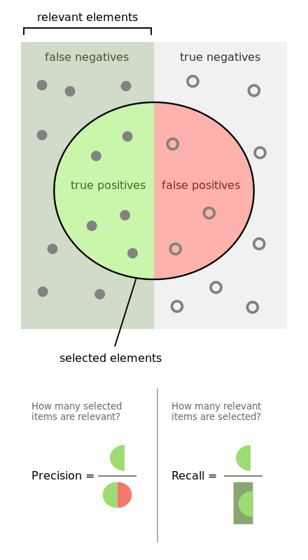
In layman’s terms, precision asks the question: “of all the examples I guessed were positive, what proportion were actually positive?” and recall asks the question: “of all the examples that were actually positive, what proportion did I correctly guess as positive?”
The F-beta score (a generalization of the traditional F1 score) is a weighted average of precision and recall, also measured on a scale of 0 to 1:

When beta = 1, we get the standard F1 measure of 2 * (precision * recall) / (precision + recall). In general, beta represents how many times more important recall should be than precision. For our fraud detection model, we’ll use the F1 score as our high score to track, but we’ll log the precision and recall scores as well to check the balance. This is our f1-test-fn:
defn f-beta
  "F-beta score, default uses F1"
  ([precision recall] (f-beta precision recall 1))
  ([precision recall beta]
    (let [beta-squared (* beta beta)]
      (* (+ 1 beta-squared)
         (try                         ;; catch divide by 0 errors
           (/ (* precision recall)
              (+ (* beta-squared precision) recall))
         (catch ArithmeticException e
           0))))))


(defn f1-test-fn
  "Test function that takes in two map arguments, global info and local epoch info.
   Compares F1 score of current network to that of the previous network,
   and returns map:
    {:best-network? boolean
     :network (assoc new-network :evaluation-score-to-compare)}"
  [;; global arguments
   {:keys [batch-size context]}
   ;per-epoch arguments
   {:keys [new-network old-network test-ds]} ]
  (let [batch-size (long batch-size)
        test-results (execute/run new-network test-ds
                                 :batch-size batch-size
                                 :loss-outputs? true
                                 :context context)
         ;;; test metrics
         test-actual (mapv #(vec->label [0.0 1.0] %) (map :label test-ds))
         test-pred (mapv #(vec->label [0.0 1.0] % [1 0.9]) (map :label test-results))

         precision (metrics/precision test-actual test-pred)
         recall (metrics/recall test-actual test-pred)
         f-beta (f-beta precision recall)

         ;; if current f-beta higher than the old network's, current is best network
         best-network? (or (nil? (get old-network :cv-score))
                          (> f-beta (get old-network :cv-score)))
         updated-network (assoc new-network :cv-score f-beta)
         epoch (get new-network :epoch-count)]

    (experiment-train/save-network updated-network network-file)
    (log (str "Epoch: " epoch "\n"
              "Precision: " precision  "\n"
              "Recall: " recall "\n"
              "F1: " f-beta "\n\n"))
    {:best-network? best-network?
     :network updated-network}))
The function runs the current network on the test set, calculates the F1 score, and updates/saves the network accordingly. It also prints out our evaluation metrics at each epoch. If we run (train) in the REPL now, we get a high score that something that looks like this:
Epoch: 30
Precision: 0.2515923566878981
Recall: 0.9186046511627907
F1: 0.395
Data Augmentation
Here’s the problem. Remember how I said our highly imbalanced dataset was going to cause issues for us later? The model currently does not have enough positive examples to learn from. When we call experiment-util/infinite-class-balanced-dataset in our train function, we’re actually creating hundreds of copies of each positive training instance to balance out the dataset. As a result, the model is effectively memorizing those feature values and not actually learning the distinction between the classes.
One way around this problem is through data augmentation, in which we generate additional, artificial data based on the examples we already have. In order to create realistic positive training examples, we are going to add random amounts of noise to the feature vectors of each of our existing positive examples. The amount of noise we add will be dependent on the variance of each feature across the positive class, such that features with a large variance will be augmented with a large amount of noise, and vice versa for features with small variances.
Here is our code for data augmentation:
(defonce get-scaled-variances
  (memoize
    (fn []
      (let [{positives true negatives false} (group-by #(= (:label %) [0.0 1.0]) (create-dataset))
            pos-data (mat/matrix (map #(:data %) positives))
            variances (mat/matrix (map #(matstats/variance %) (mat/columns pos-data)))
            scaled-vars (mat/mul (/ 5000 (mat/length variances)) variances)]
        scaled-vars))))


(defn add-rand-variance
  "Given vector v, add random vector based off the variance of each feature"
  [v scaled-vars]
  (let [randv (map #(- (* 2 (rand %)) %) scaled-vars)]
    (mapv + v randv)))


(defn augment-train-ds
  "Takes train dataset and augments positive examples to reach 50/50 balance"
  [orig-train]
  (let [{train-pos true train-neg false} (group-by #(= (:label %) [0.0 1.0]) orig-train)
        pos-data (map #(:data %) train-pos)
        num-augments (- (count train-neg) (count train-pos))
        augments-per-sample (int (/ num-augments (count train-pos)))

        augmented-data (apply concat (repeatedly augments-per-sample
                                        #(mapv (fn [p] (add-rand-variance p (get-scaled-variances))) pos-data)))
        augmented-ds (mapv (fn [d] {:data d :label [0 1]}) augmented-data)]
    (shuffle (concat orig-train augmented-ds))))
augment-train-ds takes our original train dataset, calculates the number of augmentations that have to be made to reach a 50/50 class balance, and applies those augmentations to our existing samples by adding a random noise vector (add-rand-variance) based on the allowed variance (get-scaled-variances). In the end, we concatenate the augmented examples back in to the original dataset and return the balanced dataset.
During training, the model will be seeing an unrealistically large amount of positive examples, while the test set will still be only 0.172% positives. As a result, while the model may be able to learn the differences between the two classes better, it will over-predict positive examples during testing. In order to fix this, we can require a higher threshold of certainty to predict “positive” during testing. In other words, instead of requiring the model to be at least 50% certain that an example is positive in order to classify it as such, we can require it to be at least 70% certain. After some testing, I found the optimal value to be set at 90%. The code for this can be found in the vec->label function in the source code, and is called on line 31 of the f1-test-fn.
Using the new, augmented dataset for training, our high scores look something like this:
Epoch: 25
Precision: 0.8658536585365854
Recall: 0.8255813953488372
F1: 0.8452380952380953
Much better!
Conclusion
As always, the model can still be improved. Here are a few ideas for next steps:
- Are all the PCA features informative? Take a look at the distribution of values for positive and negative examples across the features, and drop any features that do not help distinguish between the two classes.
- Are there other neural net architectures, activation functions, etc. that perform better?
- Are there different data augmentation techniques that would perform better?
- How does model performance in Cortex compare to Keras/Tensorflow/Theano/Caffe?
The source code for the project can be found in its entirety here. I encourage you to try some of these next steps, test out new datasets, and explore different network architectures (we have a great image classification example for reference on conv nets). Cortex is pushing towards its 1.0 release, so if you have any thoughts, recommendations, or feedback, be sure to let us know. Happy hacking!

WorksHub
Jobs
Locations
Articles
Ground Floor, Verse Building, 18 Brunswick Place, London, N1 6DZ
108 E 16th Street, New York, NY 10003
Subscribe to our newsletter
Join over 111,000 others and get access to exclusive content, job opportunities and more!