Quantum Computing and AI Tie the Knot
Jason Roell
13 Apr 2018
•
7 min read

In 2018, quantum technicians and daring developers are using quantum algorithms to transform the field of artificial neural network optimization: the bees knees of machine learning and AI. So we can say with some confidence that thanks to quantum algorithms, the future of quantum computing and artificial intelligence are hopelessly entangled. So let’s take a deep dive into the quantum algorithms that are making waves in the digital age. I’ll be paying special attention to quantum annealing (rhymes with feeling), a unique animal that seems to thrive in an AI-rich area where classical algorithms often struggle or altogether fail: training artificial neural networks.
Trouble training your neural net? Join the club…
Rather amazingly, you can train artificial neural nets such as RNNs and CNNs to get wise and not make the same mistake twice. It’s this power to follow Esther Dyson’s advice that makes neural nets the intelligence engine that drives machine learning and AI. That said, training neural networks is a notoriously tricky task. But this hasn’t stopped researchers and coders from working furiously over the last few years to find new ways to reduce training errors with bleeding-edge optimization algorithms. The first stab at the error-reduction problem is best known as hill climbing. Let’s run through it.
Hill climbing
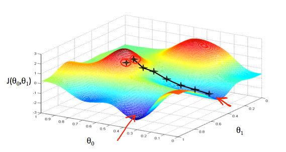
Optimization algorithms that belong to the hill climbing club always check for the gradient (more or less the steepness of a graphed function’s slope) before making their next move. But this runs a real risk of missing out on the real action going on in the graph’s landscape. Two enemies hill climbers often find themselves facing are the plateau problem and the local minima problem. In a word, these problems are the hiker’s equivalent to getting lost in a mirage-riddled desert, or getting stuck in a small muddy valley. But let’s dig deeper…
The plateau problem
When an optimization process enters a plateau, it means it’s getting roughly the same output (y) for every input (x). Because the slope of the function is at or near zero for long flat stretches, an optimization algorithm can run out of time before it finds the edge. And like a shimmering desert mirage, the long stretches of flat function can create the illusion that you’ve reached an optimal state (in this case the global minimum) when you’re nowhere near it.
Cost
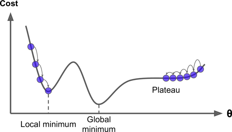
The local minima problem
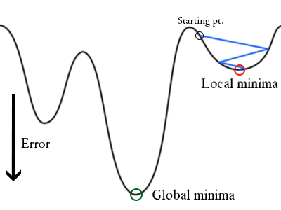
A local minimum is a relatively small valley in the graph of a function whose deepest and most important valley lies elsewhere. You can think of the optimization process (when it’s searching for the lowest value in a function) as a beach ball: it will roll downhill and eventually stop at the lowest point in the immediate landscape, even if there’s a much deeper valley on the other side of a nearby hill. That’s the problem.
The most exciting solution
There are a number of alternatives to conventional hill climbing that can help you get out of the dreaded valleys posed by the local minima problem and the desert mirages posed by the plateau problem. But for the purposes at hand, let’s just focus on the most exciting solution: simulated annealing. This is a wild breed of optimization animal that is tackling valleys and plateaus in a computationally clever way that’s well worth at least a couple paragraphs of pondering…
The hottest and coolest classical optimization algorithm around
To cut to the chase, simulated annealing steals from physics to tie time and temperature together in a single elegant algorithm. Yes, you read that right: an algorithm with a temperature parameter. When you run a simulated annealing algorithm, it begins with a completely random, frenetic series of selections from the entire landscape of the function at hand. This is the hot phase of the process. But as the temperature parameter drops with time, the random selections cover an ever-narrower range of the landscape. Finally, we enter the cool phase of the process as the algorithm begins to home in on (with a little luck) the deepest valley or the highest peak, where the holy grail of optimization lies: the global minimum or maximum.
Although the code found in simulated annealing algorithms generally contains some heavy math, the underlying connection between time and temperature is quite easy to grasp. Just picture something hot moving wildly throughout an unknown landscape, hitting everything in sight and reporting back a very rough picture of the lay of the land. Then you can think of progressively colder things moving ever-more slowly and cautiously through an ever-narrower region of the landscape, documenting the details as they creep further down into the deepest valley or up onto the highest peak… Okay, if you’re still not sure what on earth I’m talking about, here’s an excellent animation that should do the trick.
Quantum annealing (oh, what a feeling)
Simulated annealing can often get you out of a pinch when the other alternatives to conventional hill climbing come up short. But it’s an extremely specialized approach, and it suffers from at least one chilling drawback: you have to run the algorithm for an infinite amount of time to smoothly reach absolute zero and thus guarantee that you reach the true global minimum or maximum in the energy landscape. Since you probably don’t have an eternity to spare, you will never really know if your optimization solution is caught in yet another trap.
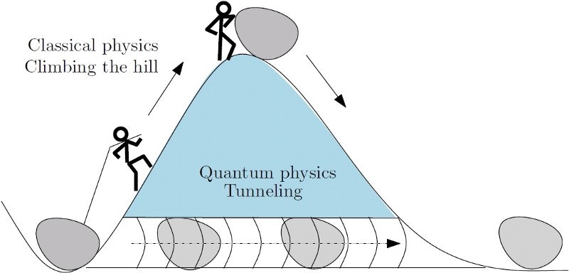
Enter quantum annealing. First, it’s important to keep in mind that quantum annealing algorithms in their basic form are remarkably similar to simulated annealing algorithms. Why? Because quantum tunneling strength plays the same role in quantum annealing as temperature does in simulated annealing. As time passes, the quantum tunneling strength in the quantum annealer drops dramatically, just as the temperature in the simulated annealer drops dramatically. It’s also easy to visualize the similarity between tunneling-strength and temperature. As time passes and quantum tunneling strength decreases, the system gets cozier and cozier with each progressively deeper valley in the energy landscape, and less and less inclined to tunnel its way out. Eventually, it gives up tunneling altogether when it finds itself (ideally) at the bottom of the deepest and coziest valley in the energy landscape (AKA the global minimum).
Not your grandmother’s quantum computer
The first difference your bound to notice between relatively conventional quantum computers and quantum annealing computers is the number of qubits they use. While the state-of-the-art in conventional quantum computers is pushing a few dozen qubits in 2018, the leading quantum annealer has more than 2000 qubits. Of course, the trade-off is that quantum annealers are not universal but specialized quantum computers that technically tackle only optimization problems and sampling problems. Because solving optimization problems is considered one of the key paths to the AI promised land, I’m going to focus on it from here on out.
A dizzying state of disarray
Before we apply the quantum annealing algorithm to the pool of qubits in our quantum annealer, they’re a mess: a maximally cloudy and unconnected configuration. This means we start out knowing nothing about the quantum system, which may be in any of 2^n different states (where n is the number of qubits). For a quantum annealer with 2000 qubits, that’s a crazy number of possible states. If you have any doubts about that, try plugging 2²⁰⁰⁰ into your favorite calculator for a second opinion.
The quantum wishing well
Individual qubits always start out in an initial state of cloudy superposition that places them at the minimum possible energy. Physicists like to visualize this lowest-energy state as the bottom of a quantum potential well that looks sort of like a big letter U.
U
0/1
Then quantum annealing comes along and forces the state of superposition into two halves, two states, two bottoms of the well: 0 and 1. The result looks more like a big letter W:
W
0 1
The next step for the quantum annealer is to start loading the dice to favor the house in the quantum probability game.
Biases
With the help of an applied magnetic field, the quantum annealer nudges each qubit into being heavily biased toward 0 or 1: favoring either the first or the second dip in the W above.
Couplings
While quantum annealers are loading the dice (that is, individual qubits) with biases via magnetic fields, they are also busy tying together pairs of dice with theoretical threads via couplers. Specifically, a coupler can do one of two things. It can guarantee that a pair of qubits are always in the same state: either both 0 or both 1. Or it can ensure that two neighboring qubits are always in the opposite state: 0 and 1, or 1 and 0. The quantum coupler uses (surprise, surprise) quantum entanglement to tie qubits together and create the couplings.
Sculpting an energy landscape
As an aspiring developer working with a quantum annealer, it’s your job to essentially load all the quantum dice by coding a collection of biases and couplings that define the optimization problem you want your trusty annealer to solve. Another way to look at it is that you are sculpting, or at least generating, a sophisticated energy landscape of peaks and valleys that represent all possible outcomes in your optimization problem. Then you are setting the quantum annealer loose to search and ferret out the very bottom of that energy landscape’s deepest valley, which corresponds to the optimal solution. If you’re consistently successful, then your quantum annealing prowess may help power a new generation of machine learning and AI for posterity.
Quantum computing and AI news
On August 31st, 2017, the Universities Space Research Association (USRA) announced that in partnership with NASA and Google it had upgraded the quantum annealing computer at the Quantum Artificial Intelligence Lab (Quantum AI Lab) to a D-Wave 2000Q. With nearly twice as many qubits as its predecessor and a new knack for “adiabatic quantum computing,” the latest D-Wave is going after bigger fish in the optimization-problem pond. The USRA team has even got their eye on using quantum algorithms and the D-Wave to tackle “challenging computational problems involved in NASA missions.” Partner Google, on the other hand, has their eye on AI:
"We are particularly interested in applying quantum computing to artificial intelligence and machine learning."
But it’s not just Google and NASA that have access to the Quantum AI Lab. Believe it or not, you may too. If you’re a qualified candidate, you might just get some quality time with the latest D-Wave to try out your genius idea. In the Lab’s own words, “the call is open.”
If you liked this article I would be super excited if you could share with your curious friends. I’ve got much more like it over at my personal blog jasonroell
Anyway, thanks again for reading have a great day!

WorksHub
Jobs
Locations
Articles
Ground Floor, Verse Building, 18 Brunswick Place, London, N1 6DZ
108 E 16th Street, New York, NY 10003
Subscribe to our newsletter
Join over 111,000 others and get access to exclusive content, job opportunities and more!